AL – Opérations sur matrices
Le déterminant d’une matrice carrée
-
Le déterminant de la matrice \(A \in M_{2}(\mathbb{R})\) est un scalaire \(\operatorname{det}(A) \in \mathbb{R}\), il se note :
\(\operatorname{det}(A)=\left|\begin{array}{cc}a & b \\ c & d\end{array}\right|\) et est définit par \(\operatorname{det}(A)=a d-b c\), où \(A=\left[\begin{array}{ll}a & b \\ c & d\end{array}\right]\)
-
Le déterminant de la matrice \(A \in M_{n}(\mathbb{R})\) est un scalaire \(\operatorname{det}(A) \in \mathbb{R}\), il se note
$$
\operatorname{det}(A)=\left|\begin{array}{ccc}
a_{11} & \ldots & a_{1 n} \\
a_{21} & \ldots & a_{2 n} \\
\vdots & \ddots & \vdots \\
a_{n 1} & \ldots & a_{n n}
\end{array}\right|
$$
Il est donné par \(\operatorname{det}(A)=\sum_{j=1}^{n} a_{i j}(-1)^{i+j} \operatorname{det}\left(A_{i j}\right)\)
Où \(A_{i j}\) la matrice carrée de taille \(n-1\) obtenue en supprimant dans \(A\) la ligne \(i\) et la colonne \(j\).
Technique de calcul
Pour développer un déterminant d’ordre \(n\) sous la forme d’une somme de \(n\) déterminants d’ordre \(n-1\), suivant une ligne ou suivant une colonne. On développera les \(n\) déterminants d’ordre \(n-1\) sous la forme d’une somme de \(n-1\) déterminants d’ordre \(n-2\). On continue jusqu’à obtenir des sommes de déterminants d’ordre 2 que l’on sait calculer. Ci-après la technique de calcul le déterminant de dimension 3 :
Le développement en ligne ou en colonne :
$$
\begin{aligned}
& \left\{\begin{array}{l}
a\left|\begin{array}{ll}
e & f \\
h & k
\end{array}\right|-d\left|\begin{array}{ll}
b & c \\
h & k
\end{array}\right|+g\left|\begin{array}{ll}
b & c \\
e & f
\end{array}\right| \\
\text { (développement par rapport à la première colonne) }
\end{array}\right. \\
& \left\{-b\left|\begin{array}{ll}
d & f \\
g & k
\end{array}\right|+e\left|\begin{array}{ll}
a & c \\
g & k
\end{array}\right|-h\left|\begin{array}{ll}
a & c \\
d & f
\end{array}\right|\right. \\
& \text { (développement par rapport à la deuxième colonne) } \\
& c\left|\begin{array}{ll}
d & e \\
g & h
\end{array}\right|-f\left|\begin{array}{ll}
a & b \\
g & h
\end{array}\right|+k\left|\begin{array}{ll}
a & b \\
d & e
\end{array}\right| \\
& \text { (développement par rapport à la troisième colonne) }
\end{aligned}
$$
et de la même façon
$$
\begin{aligned}
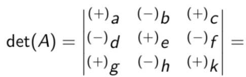
& \operatorname{det}(A)=\left|\begin{array}{lll}
(+) a & (-) b & (+) c \\
(-) d & (+) e & (-) f \\
(+) g & (-) h & (+) k
\end{array}\right|= \\
& a\left|\begin{array}{ll}
e & f \\
h & k
\end{array}\right|-b\left|\begin{array}{ll}
d & f \\
g & k
\end{array}\right|+c\left|\begin{array}{ll}
d & e \\
g & h
\end{array}\right| \\
& \text { (développement par rapport à la première ligne) } \\
& -d\left|\begin{array}{ll}
b & c \\
h & k
\end{array}\right|+e\left|\begin{array}{ll}
a & c \\
g & k
\end{array}\right|-f\left|\begin{array}{ll}
a & b \\
g & h
\end{array}\right| \\
& \text { (développement par rapport à la deuxième ligne) } \\
& g\left|\begin{array}{ll}
b & c \\
e & f
\end{array}\right|-h\left|\begin{array}{ll}
a & c \\
d & f
\end{array}\right|+k\left|\begin{array}{ll}
a & b \\
d & e
\end{array}\right| \\
& \text { (développement par rapport à la troisième ligne) }
\end{aligned}
$$
\(\textbf{Exemple 3.1}\) Soit \(A=\left[\begin{array}{ccc}-2 & 2 & -3 \\ -1 & 1 & 3 \\ 2 & 0 & -1\end{array}\right]\), alors :
$$
\begin{aligned}
\operatorname{det}(A)=\left|\begin{array}{ccc}
-2 & 2 & -3 \\
-1 & 1 & 3 \\
2 & 0 & -1
\end{array}\right| & =(-2)\left|\begin{array}{cc}
1 & 3 \\
0 & -1
\end{array}\right|-(2)\left|\begin{array}{cc}
-1 & 3 \\
2 & -1
\end{array}\right|+(-3)\left|\begin{array}{cc}
-1 & 1 \\
2 & 0
\end{array}\right| \\
& =(-2)[(1)(-1)-(3)(0)]+(-2)[(-1)(-1)-(2)(3)]+ \\
& =(-2)(-1)-(2)(-5)+(-3)(-2) \\
& =2+10+6=18
\end{aligned}
$$
Les 3 Opérations élémentaires (OE) sur les lignes et les colonnes
À partir de maintenant, on note \(C_{i}\) (resp. \(L_{i}\) ) la \(i^{e}\) colonne(resp. ligne) d’une matrice
Définition 3.2: opérations élémentaires sur les lignes (colonnes)
-
Remplacer une ligne (colonne) par la ligne (colonne) obtenue en lui ajoutant un multiple d’une autre ligne (colonne).
Échanger deux lignes (colonnes).
Multiplier tous les coefficients d’une ligne (colonne) par une constante non nulle.
\(\textbf{Propriétés:}\)
Le symbole \(\rightleftharpoons\) définit l’échange entre 2 lignes (ou colonnes)
-
On ne change pas un déterminant en ajoutant à une colonne (resp. ligne) une combinaison linéaire des autres colonnes (resp. lignes )
(opérations élémentaires sur les lignes et les colonnes)
\(\forall \lambda, \mu \in \mathbb{R}:\)
\(\left|\begin{array}{ccccccccc}a_{11} & \ldots & a_{1 j} & \ldots & a_{i k} & \ldots & a_{1 t} & \ldots & a_{1 n} \\ a_{21} & \ldots & a_{2 j} & \ldots & a_{2 k} & \ldots & a_{2 t} & \ldots & a_{2 n} \\ \vdots & & \vdots & & \vdots & \ldots & \vdots & \ldots & \vdots \\ a_{n 1} & \ldots & a_{n j} & \ldots & a_{n k} & \ldots & a_{n t} & \ldots & a_{n n}\end{array}\right|=\left|\begin{array}{ccccccc}a_{11} & \ldots & a_{1 j}+\lambda a_{1 k}+\mu a_{1 t} & \ldots . & a_{i k} & \ldots & a_{1 n} \\ a_{21} & \ldots & a_{2 j}+\lambda a_{2 k}+\mu a_{2 t} & \ldots & a_{2 k} & \ldots & a_{2 n} \\ \vdots & & \vdots & & \vdots & & \vdots \\ a_{n 1} & \ldots & a_{n j}+\lambda a_{n k}+\mu a_{n t} & \ldots & a_{n k} & \ldots & a_{n n}\end{array}\right|\)
\(C_{j} \rightleftharpoons C_{j}+\lambda C_{k}+\mu C_{t} \Longrightarrow\) Ce changement n’affecte pas la valeur du déterminant.
-
On multiple le déterminant par -1 si on inverse deux colonnes (lignes) du déterminant.
$$
\begin{aligned}
& C_{i} \rightleftharpoons C_{j} \Longrightarrow \operatorname{det}(A)=-\operatorname{det}\left(A^{\prime}\right) \\
& L_{i} \rightleftharpoons L_{j} \Longrightarrow \operatorname{det}(A)=-\operatorname{det}\left(A^{\prime}\right)
\end{aligned}
$$
où \(A^{\prime}\) est la matrice après l’opération.
-
On multiple le déterminant par \(k\) si on multiplie une colonne (ligne) d’un déterminant par \(k \in \mathbb{R}\).
$$
C_{i} \rightleftharpoons K \cdot C_{i} \Longrightarrow \operatorname{det}\left(A^{\prime}\right)=k \cdot \operatorname{det}(A)
$$
où \(A^{\prime}\) est la matrice obtenue à partir de \(A\) en multipliant le colonne \(C_{i}\) par \(k\).
-
Le déterminant d’une matrice est nul si tous les éléments d’une ligne (colonne) du déterminant sont nuls. Aussi :
$$
\begin{array}{ll}
\exists C_{i}, C_{j} ; & C_{i}=C_{j} \Longrightarrow \operatorname{det}(A)=0 . \\
\exists L_{i}, L_{j} ; & L_{i}=L_{j} \Longrightarrow \operatorname{det}(A)=0 .
\end{array}
$$
\(\textbf{Exemple 3.2}\)
Soit
$$
A=\left[\begin{array}{ccc}
1 & 3 & -3 \\
0 & 0 & 0 \\
2 & -1 & 9
\end{array}\right] \Rightarrow \operatorname{det}(A)=\left|\begin{array}{ccc}
1 & 3 & -3 \\
0 & 0 & 0 \\
2 & -1 & 9
\end{array}\right|
$$
En calculant le déterminant par la deuxième ligne, on obtient \(\operatorname{det}(A)=0\).
\(\textbf{Exemple 3.3}\) Soit le déterminant de la matrice \(A: \operatorname{det}(A)=\left|\begin{array}{lll}2 & 3 & -1 \\ 0 & 4 & -2 \\ 2 & 3 & -1\end{array}\right|\)
On ajoute \(-L_{3}\) à \(L_{1}\) (i.e. \(\left.L_{1} \rightleftharpoons L_{1}-L_{3}\right)\), on obtient :
$$
\operatorname{det}(A)=\left|\begin{array}{ccc}
0 & 0 & 0 \\
0 & 4 & -2 \\
2 & 3 & -1
\end{array}\right|=0
$$
-
Le déterminant est linéaire par rapport à chacune de ses colonnes ou de ses lignes : pout tout \(1 \leq j \leq n\) et \(\lambda, \mu \in \mathbb{R}\) :
\(\left|\begin{array}{ccccc}a_{11} & \ldots & \lambda a_{1 j}+\mu b_{1 j} & \ldots & a_{1 n} \\ \vdots & & \vdots & & \vdots \\ a_{n 1} & \ldots & \lambda a_{n j}+\mu b_{n j} & \ldots & a_{n n}\end{array}\right|=\left|\begin{array}{ccccc}a_{11} & \ldots & \lambda a_{1 j} & \ldots & a_{1 n} \\ \vdots & & \vdots & & \vdots \\ a_{n 1} & \ldots & \lambda a_{n j} & \ldots & a_{n n}\end{array}\right|+\left|\begin{array}{ccccc}a_{11} & \ldots & \mu b_{1 j} & \ldots & a_{1 n} \\ \vdots & & \vdots & & \vdots \\ a_{n 1} & \ldots & \mu b_{n j} & \ldots & a_{n n}\end{array}\right|\)
Aussi pour tout \(1 \leq i \leq n\) :
\(\left|\begin{array}{ccc}a_{11} & \ldots & a_{1 n} \\ \vdots & & \vdots \\ \lambda a_{i 1}+\mu b_{i 1} & \ldots & \lambda a_{i n}+\mu b_{i n} \\ \vdots & & \vdots \\ a_{n 1} & \ldots & a_{n n}\end{array}\right|=\left|\begin{array}{ccc}a_{11} & \ldots & a_{1 n} \\ \vdots & & \vdots \\ \lambda a_{i 1} & \ldots & \lambda a_{i n} \\ \vdots & & \vdots \\ a_{n 1} & \ldots & a_{n n}\end{array}\right|+\left|\begin{array}{ccc}a_{11} & \ldots & a_{1 n} \\ \vdots & & \vdots \\ \mu b_{i 1} & \ldots & \mu b_{i n} \\ \vdots & & \vdots \\ a_{n 1} & \ldots & a_{n n}\end{array}\right|\)
\(\textbf{Exemple 3.4}\)On \(a\) :
$$
\underbrace{\left|\begin{array}{cc}
2+3 & 2 \\
5+2 & 1
\end{array}\right|}_{=-9}=\underbrace{\left|\begin{array}{ll}
2 & 2 \\
5 & 1
\end{array}\right|}_{=-8}+\underbrace{\left|\begin{array}{ll}
3 & 2 \\
2 & 1
\end{array}\right|}_{=-1}, \quad \underbrace{\left|\begin{array}{cc}
2+3 & 2+1 \\
5 & 1
\end{array}\right|}_{=-10}=\underbrace{\left|\begin{array}{cc}
2 & 2 \\
5 & 1
\end{array}\right|}_{=-8}+\underbrace{\left|\begin{array}{ll}
3 & 1 \\
5 & 1
\end{array}\right|}_{=-2}
$$
-
Si \(A=\left[a_{i j}\right] \in M_{n}(\mathbb{R})\) est une matrice carrée triangulaire ou diagonale alors :
$$
\operatorname{det}(A)=\prod_{i=1}^{n} a_{i i}
$$
Les opérations sur des déterminants :
Soient \(A, B \in M_{n}(\mathbb{R})\) et \(r \in \mathbb{R}\), alors :
-
\(\operatorname{det}(A \times B)=\operatorname{det}(A) \cdot \operatorname{det}(B)\).
\(\operatorname{det}(r \cdot A)=r^{n} \cdot \operatorname{det}(A)\)
\(\operatorname{det}\left(A^{T}\right)=\operatorname{det}(A)\).
L’inverse d’une matrice carrée
On dit qu’une matrice carrée \(A \in M_{n}(\mathbb{R})\) est inversible s’il existe une matrice \(B \in M_{n}(\mathbb{R})\) telle que
$$
A B=B A=\mathbb{I}_{n}
$$
On dit que \(B\) est la matrice inverse de \(A\), et on note \(B=A^{-1}\). Donc
$$
A A^{-1}=A^{-1} A=\mathbb{I}_{n} .
$$
Une matrice carrée qui n’est pas inversible est dite non inversible ou singulière
\(\textbf{Exemple 4.1}\) On trouve évident que \(\mathbb{I}_{n} \mathbb{I}_{n}=\mathbb{I}_{n}\). Donc, \(\mathbb{I}_{n}^{-1}=\mathbb{I}_{n}\).
$$
\mathbb{I}_{n} \mathbb{I}_{n}=\left[\begin{array}{ccccc}
1 & 0 & 0 & \ldots & 0 \\
0 & 1 & 0 & \ldots & 0 \\
0 & 0 & 1 & \ldots & 0 \\
\vdots & \vdots & \vdots & \ddots & \vdots \\
0 & 0 & 0 & \ldots & 1
\end{array}\right]\left[\begin{array}{ccccc}
1 & 0 & 0 & \ldots & 0 \\
0 & 1 & 0 & \ldots & 0 \\
0 & 0 & 1 & \ldots & 0 \\
\vdots & \vdots & \vdots & \ddots & \vdots \\
0 & 0 & 0 & \ldots & 1
\end{array}\right]=\left[\begin{array}{ccccc}
1 & 0 & 0 & \ldots & 0 \\
0 & 1 & 0 & \ldots & 0 \\
0 & 0 & 1 & \ldots & 0 \\
\vdots & \vdots & \vdots & \ddots & \vdots \\
0 & 0 & 0 & \ldots & 1
\end{array}\right] .
$$
\(\textbf{Exemple 4.2}\) Soit \(A=\left[\begin{array}{cc}2 & 3 \\ -3 & -7\end{array}\right]\) et \(B=\left[\begin{array}{cc}-7 & -5 \\ 3 & 2\end{array}\right]\), on \(a\) :
$$
\begin{aligned}
& A B=\left[\begin{array}{cc}
2 & 3 \\
-3 & -7
\end{array}\right]\left[\begin{array}{cc}
-7 & -5 \\
3 & 2
\end{array}\right]=\left[\begin{array}{ll}
1 & 0 \\
0 & 1
\end{array}\right] \\
& \left.B A=\left[\begin{array}{cc}
-7 & -5 \\
3 & 2
\end{array}\right]\left[\begin{array}{cc}
2 & 3 \\
-3 & -7
\end{array}\right]=\left[\begin{array}{ll}
1 & 0 \\
0 & 1
\end{array}\right]\right\} \Rightarrow B=A^{-1} .
\end{aligned}
$$
Calculer l’inverse d’une matrice carrée
\(\textbf{Théorème 4.1}\) Soit \(A \in M_{n}(\mathbb{R}), A\) est inversible si et seulement si
$$
\operatorname{det}(A) \neq 0 .
$$
\(\textbf{Théorème 4.2}\) Si \(A=\left[\begin{array}{ll}a & b \\ c & d\end{array}\right] \in M_{2}(\mathbb{R})\) et \(\operatorname{det}(A) \neq 0\), on a :
$$
A^{-1}=\frac{1}{\operatorname{det}(A)} \cdot\left[\begin{array}{cc}
d & -b \\
-c & a
\end{array}\right]
$$
\(\textbf{Démonstration}\) On cherchera une matrice carrée \(B \in M_{2}(\mathbb{R})\) telle que
$$
A B=B A=\mathbb{I}_{2}
$$
On pose \(: B=\left[\begin{array}{ll}x & y \\ z & t\end{array}\right] \Rightarrow A B=\left[\begin{array}{ll}a x+b z & a y+b t \\ c x+d z & c y+d t\end{array}\right]\)
$A B=\mathbb{I}_{2} \Leftrightarrow\left[\begin{array}{ll}a x+b z & a y+b t \\ c x+d z & c y+d t\end{array}\right]=\left[\begin{array}{cc}1 & 0 \\ 0 & 1\end{array}\right] \Leftrightarrow\left\{\begin{array}{l}a x+b z=1 \\ c x+d z=0 \\ a y+b t=0 \\ c y+d t=1\end{array}\right.$
Alors on obtient deux systèmes de deux équations :
$$
\text { (I) }:\left\{\begin{array}{l}
a x+b z=1 \\
c x+d z=0
\end{array},(\mathrm{II}):\left\{\begin{array}{l}
a y+b t=0 \\
c y+d t=1
\end{array}\right.\right.
$$
Ces deux systèmes admettent une unique solution puisque \(a d \neq b c\).
Après calcul on a : \(\left\{\begin{array}{l}x=\frac{d}{\operatorname{det}(A)} \\ z=\frac{-c}{\operatorname{det}(A)}\end{array}\right.\) et \(\left\{\begin{array}{l}y=\frac{-b}{\operatorname{det}(A)} \\ t=\frac{a}{\operatorname{det}(A)}\end{array}\right.\)
Ainsi, \(B=\left[\begin{array}{cc}\frac{d}{\operatorname{det}(A)} & \frac{-b}{\operatorname{det}(A)} \\ \frac{-c}{\operatorname{det}(A)} & \frac{a}{\operatorname{det}(A)}\end{array}\right]=\frac{1}{\operatorname{det} A} \cdot\left[\begin{array}{cc}d & -b \\ -c & a\end{array}\right]\).
matrice cofacteur
On appelle matrice des cofacteurs (ou comatrice) d’une matrice \(A \in M_{n}(\mathbb{R})\), et on note \(\operatorname{com}(A)\), la matrice de coefficients
$$
c_{i j}=(-1)^{i+j} \operatorname{det}\left(A_{i j}\right)
$$
où \(A_{i j}\) est la matrice carrée de dimension \(n-1\) obtenue en supprimant dans \(A\) la ligne \(i\) et la colonne \(j\).
\(\textbf{Exemple 4.3}\) Soit \(B=\left[\begin{array}{ccc}1 & 2 & 3 \\ 0 & 1 & 2 \\ -1 & -4 & -1\end{array}\right]\)
$$
\operatorname{com}(B)=\left[\begin{array}{ccc}
+\left|\begin{array}{cc}
1 & 2 \\
-4 & -1
\end{array}\right| & -\left|\begin{array}{cc}
0 & 2 \\
-1 & -1
\end{array}\right| & +\left|\begin{array}{cc}
0 & 1 \\
-1 & -4
\end{array}\right| \\
-\left|\begin{array}{cc}
2 & 3 \\
-4 & -1
\end{array}\right| & +\left|\begin{array}{cc}
1 & 3 \\
-1 & -1
\end{array}\right| & -\left|\begin{array}{cc}
1 & 2 \\
-1 & -4
\end{array}\right| \\
+\left|\begin{array}{ll}
2 & 3 \\
1 & 2
\end{array}\right| & -\left|\begin{array}{cc}
1 & 3 \\
0 & 2
\end{array}\right| & +\left|\begin{array}{cc}
1 & 2 \\
0 & 1
\end{array}\right|
\end{array}\right]=\left[\begin{array}{ccc}
7 & -2 & 1 \\
-10 & 2 & 2 \\
1 & -2 & 1
\end{array}\right]
$$
\(\textbf{Théorème 4.3}\) Si \(A \in M_{n}(\mathbb{R})\) est inversible alors :
$$
A^{-1}=\frac{1}{\operatorname{det}(A)} \cdot(\operatorname{com}(A))^{T}
$$
\(\textbf{Exemple 4.4}\) Pour la matrice \(B\) de l’exemple précédent on trouve :
$$
\operatorname{det}(B)=\left|\begin{array}{ccc}
1 & 2 & 3 \\
0 & 1 & 2 \\
-1 & -4 & -1
\end{array}\right|=(0)\left|\begin{array}{cc}
2 & 3 \\
-4 & -1
\end{array}\right|+(1)\left|\begin{array}{cc}
1 & 3 \\
-1 & -1
\end{array}\right|-(2)\left|\begin{array}{cc}
1 & 2 \\
-1 & -4
\end{array}\right|=6
$$
alors \(B\) est inversible, sa matrice inverse est:
$$
B^{-1}=\frac{1}{6} \cdot\left[\begin{array}{ccc}
7 & -2 & 1 \\
-10 & 2 & 2 \\
1 & -2 & 1
\end{array}\right]^{T}=\frac{1}{6} \cdot\left[\begin{array}{ccc}
7 & -10 & 1 \\
-2 & 2 & -2 \\
1 & 2 & 1
\end{array}\right]=\left[\begin{array}{ccc}
\frac{7}{6} & \frac{-10}{6} & \frac{1}{6} \\
\frac{-2}{6} & \frac{2}{6} & \frac{-2}{6} \\
\frac{1}{6} & \frac{2}{6} & \frac{1}{6}
\end{array}\right]
$$
Propriétés
-
Si \(A\) est une matrice inversible, alors \(A^{-1}\) est inversible et :
$$
\left(A^{-1}\right)^{-1}=A
$$
-
Si \(A\) et \(B\) sont deux matrices inversibles dans \(M_{n}(\mathbb{R})\), alors \(A B\) est inversible, et l’inverse de \(A B\) est
$$
(A B)^{-1}=B^{-1} \cdot A^{-1}
$$
-
Si \(A\) est une matrice inversible, alors \(A^{T}\) l’est aussi, et l’inverse de \(A^{T}\) est la transposée de \(A^{-1}\). Autrement dit,
$$
\left(A^{T}\right)^{-1}=\left(A^{-1}\right)^{T}
$$
La matrice inverse par l’algorithme du pivot de Gauss
On crée un tableau avec à gauche la matrice à inverser, et à droite la matrice identité. On réalise ensuite une suite d’opérations élémentaires sur la matrice à inverser pour la ramener à l’identité. La même suite d’opérations élémentaires effectuée sur la matrice identité donne l’inverse de la matrice de départ.
\(\textbf{Exemple 4.4 Inversons la matrice}\)
$$
\left(\begin{array}{lll}
1 & 1 & 2 \\
1 & 2 & 1 \\
2 & 1 & 1
\end{array}\right) .
$$
L’algorithme précédent donne :
$$
\begin{aligned}
& \left(\begin{array}{lll}
1 & 1 & 2 \\
1 & 2 & 1 \\
2 & 1 & 1
\end{array}\right)\left(\begin{array}{lll}
1 & 0 & 0 \\
0 & 1 & 0 \\
0 & 0 & 1
\end{array}\right) \\
& \begin{array}{c}
L_{2}-L_{1} \rightarrow L_{2} \\
L_{3}-2 L_{1} \rightarrow L_{3}
\end{array}\left(\begin{array}{ccc}
1 & 1 & 2 \\
0 & 1 & -1 \\
0 & -1 & -3
\end{array}\right)\left(\begin{array}{rrr}
1 & 0 & 0 \\
-1 & 1 & 0 \\
-2 & 0 & 1
\end{array}\right)
\end{aligned}
$$
$$
\begin{aligned}
& L_{3}+L_{2} \rightarrow L_{3}\left(\begin{array}{ccl}
1 & 1 & 2 \\
0 & 1 & -1 \\
0 & 0 & -4
\end{array}\right)\left(\begin{array}{rrr}
1 & 0 & 0 \\
-1 & 1 & 0 \\
-3 & 1 & 1
\end{array}\right) \\
& \frac{-1}{4} L_{3} \rightarrow L_{3}\left(\begin{array}{lll}
1 & 1 & 2 \\
0 & 1 & -1 \\
0 & 0 & 1
\end{array}\right)\left(\begin{array}{rcl}
1 & 0 & 0 \\
-1 & 1 & 0 \\
3 / 4 & -1 / 4 & -1 / 4
\end{array}\right) \\
& \begin{array}{c}
L_{1}-2 L_{3} \rightarrow L_{1} \\
L_{2}+L_{3} \rightarrow L_{2}
\end{array}\left(\begin{array}{ccc}
1 & 1 & 0 \\
0 & 1 & 0 \\
0 & 0 & 1
\end{array}\right)\left(\begin{array}{rrl}
-1 / 2 & 1 / 2 & 1 / 2 \\
-1 / 4 & 3 / 4 & -1 / 4 \\
3 / 4 & -1 / 4 & -1 / 4
\end{array}\right) \\
& L_{1}-L_{2} \rightarrow L_{1}\left(\begin{array}{ccc}
1 & 0 & 0 \\
0 & 1 & 0 \\
0 & 0 & 1
\end{array}\right)\left(\begin{array}{ccc}
-1 / 4 & -1 / 4 & 3 / 4 \\
-1 / 4 & 3 / 4 & -1 / 4 \\
3 / 4 & -1 / 4 & -1 / 4
\end{array}\right)
\end{aligned}
$$
La matrice inverse est donc
$$
\left(\begin{array}{ccl}
-1 / 4 & -1 / 4 & 3 / 4 \\
-1 / 4 & 3 / 4 & -1 / 4 \\
3 / 4 & -1 / 4 & -1 / 4
\end{array}\right)
$$
Systèmes linéaires, propriétés, résolution
Une équation linéaire à \(n\) inconnues à coefficients dans \(\mathbb{R}\) : est une relation du type :
$$
a_{1} x_{1}+a_{2} x_{2}+\ldots+a_{n} x_{n}=b
$$
où tous les symboles représentent des éléments de \(\mathbb{R}\). Les constantes \(a_{1}, a_{2}, \ldots a_{n}\) sont les coefficients de l’équation. les symboles \(x_{1}, x_{2}, \ldots, x_{n}\) sont désignés comme les inconnues de l’équation.
-
Un système linéaire \(m \times n\) : est une famille de \(m\) équations linéaires à \(n\) inconnues peut être écrit sous la forme suivante :
$$
\left\{\begin{array}{c}
a_{1,1} x_{1}+a_{1,2} x_{2}+\cdots+a_{1, n} x_{n}=b_{1} \\
a_{2,1} x_{1}+a_{2,2} x_{2}+\cdots+a_{2, n} x_{n}=b_{2} \\
\vdots \\
\vdots \\
a_{m, 1} x_{1}+a_{m, 2} x_{2}+\cdots+a_{m, n} x_{n}=b_{m}
\end{array}\right.
$$
Où \(x_{1}, x_{2}, \ldots, x_{n}\) sont les inconnues et les nombres \(a_{i j},(1 \leq i \leq m, 1 \leq j \leq n)\) sont les coefficients du système.
-
Le système \((\star)\) est compatible s’il existe au moins une liste \(\left(x_{1}, x_{2}, \ldots, x_{n}\right)\) telle que toutes les relations \(\mathrm{du}(\star)\) soient satisfaites simultanément.
Résoudre \((\star)\), c’est décrire toutes les listes \(\left(x_{1}, x_{2}, \ldots, x_{n}\right)\) (s’il y en a ) qui satisfont les \(m\) relations de \((\star)\).
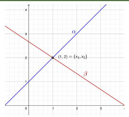
\(\textbf{Exemple 1.1}\) Résoudre le système :
\(\left(S_{1}\right) \begin{cases}x_{1}-x_{2}=-1 & \text { ‥ droite } \alpha \\ 2 x_{1}+3 x_{2}=8 & \text { … droite } \beta\end{cases}\)
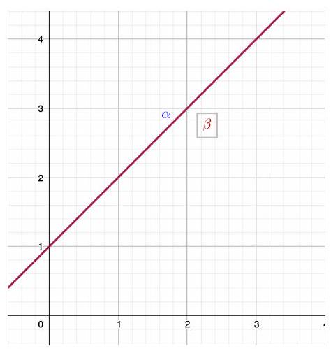
\(\textbf{Exemple 1.2}\) Résoudre le système:
\(\left(S_{2}\right)\left\{\begin{array}{cc}x_{1}-x_{2}=-1 & \text {… droite } \alpha \\ 2 x_{1}-2 x_{2}=-2 & \text {… droite } \beta\end{array}\right.\)
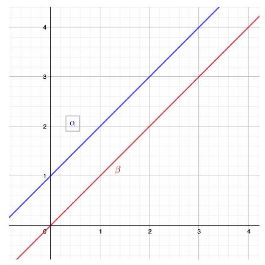
\(\textbf{Exemple 1.3}\) Résoudre le système:
\(\left(S_{3}\right)\left\{\begin{array}{cc}x_{1}-x_{2}=-1 & \ldots \text { droite } \alpha \\ x_{1}-x_{2}=0 & \text {… droite } \beta\end{array}\right.\)
\(\textbf{Exemple 1.4}\)Résoudre le système:
\(\left(S_{3}\right)\left\{\begin{array}{cc}x_{1}+x_{2}+x_3=1 & \ldots \text { Plan } \alpha \\ 2x_{1}-x_{2}=0 & \text {… Plan } \beta\end{array}\right.\)
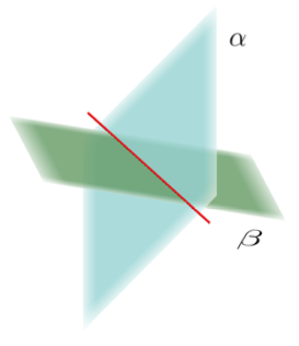
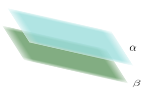
\(\textbf{Exemple 1.5}\)
\(\left(S_{5}\right)\left\{\begin{array}{cc}x_{1}+x_{2}+x_{3}=1 & \text {… Plan } \alpha \\ x_{1}+x_{2}+x_{3}=7 & \text {..P Plan } \beta\end{array}\right.\)
\(\textbf{Théorème 1.1}\) (Sur le nombre de solutions d’un système linéaire)
Tout système linéaire \(m \times n\) possède :
-
Soit aucune solution,
Soit exactement une solution,
Soit une infinité de solutions.
\(\textbf{Démonstration}\): Supposons que \((\star)\) le système linéaire \(m \times n\) ( vu plus haut) possède deux solutions distinctes, que l’on note \(\left(x_{1}, x_{2}, \ldots, x_{n}\right)\) et \(\left(y_{1}, y_{2}, \ldots, y_{n}\right)\).
On a donc
$$
\begin{aligned}
\forall j=1,2, \ldots, m: & a_{j 1} x_{1}+\ldots+a_{j n} x_{n}=b_{j} \\
& a_{j 1} y_{1}+\ldots .+a_{j n} y_{n}=b_{j}
\end{aligned}
$$
Soit \(\left(z_{1}, \ldots, z_{n}\right)\) définit comme suit
$$
\forall k=1,2, \ldots, m: z_{k}:=x_{k}+t\left(y_{k}-x_{k}\right)
$$
où \(t \in \mathbb{R}^{*}\) est fixé arbitraire.
\(\underline{\text { A voir : }}\)
\(\left(z_{1}, z_{2}, \ldots, z_{n}\right)\) est aussi une solution de \((\star)\).
\(\textbf{Remarque}\) : Si \(t \neq 0\) et \(t \neq 1:\left(z_{1}, z_{2}, \ldots, z_{n}\right)\) est distincte de \(\left(x_{1}, x_{2}, \ldots, x_{n}\right)\) et \(\left(y_{1}, y_{2}, \ldots, y_{n}\right)\) !
\(\forall j=1, . ., m\) on calcule :
$$
\begin{aligned}
& a_{j 1} z_{1}+a_{j 2} z_{2}+\ldots+a_{j n} z_{n} \ldots(*) \\
& *=a_{j 1}\left(x_{1}+t\left(y_{1}-x_{1}\right)\right)+a_{j 2}\left(x_{2}+t\left(y_{2}-x_{2}\right)\right)+\ldots+a_{j n}\left(x_{n}+t\left(y_{n}-x_{n}\right)\right) \\
&=(\underbrace{a_{j 1} x_{1}+a_{j 2} x_{2}+\ldots a_{j n} x_{n}}_{=b_{j}})+t(\underbrace{a_{j 1} y_{1}+a_{j 2} y_{2}+\ldots a_{j n} y_{n}}_{=b_{j}})-t(\underbrace{a_{j 1} x_{1}+a_{j 2} x_{2}+\ldots a_{j n} x_{n}}_{=b_{j}}) \\
&= b_{j}
\end{aligned}
$$
Donc \(\left(z_{1}, z_{2}, \ldots z_{n}\right)\) est une solution de \((\star)\).
Comme \(t \in \mathbb{R}\) est arbitraire, on peut donc construire une infinité de solutions pour \((\star)\).
Méthode Générale et Systèmes Triangulaires
Un système triangulaire est de la forme
$$
(S)\left\{\begin{array}{l}
a_{11} x_{1}+a_{12} x_{2}+\cdots+a_{1 n} x_{n}=y_{1} \\
0 \ldots \ldots \ldots \cdots \cdots \cdots \cdots \cdots a_{p n} x_{n}=y_{p}
\end{array} \Rightarrow a_{i j}=0 \text { si } i>j\right.
$$
\(\textbf{Remarque :} \) Les systèmes triangulaires sont très simple à résoudre, on utilise le terme en \(x_{1}\) de la première équation pour éliminer les termes en \(x_{1}\) des autres équations. Ensuite, on utilise le terme en \(x_{2}\) de la deuxième équation pour éliminer les termes en \(x_{2}\) des équations suivantes, et ainsi de suite, jusqu’à obtenir finalement un système triangulaire, équivalent au système de départ.
\(\textbf{But : }\) Etablir une méthode qui fonctionne toujours \(\forall\) système \(m \times n\).
\(\textbf{Idée pour la suite : }\) Essayer de rendre un système le “plus triangulaire possible”.
Opérations élémentaires
eux système \((\star),(\bar{\star})(m \times n)\) sont équivalents si ils ont le même ensemble de solutions.
But : Transformer \((\star)\) en un \((\bar{\star})\) équivalent mais plus simple à étudier. Théorème 3.1
Si \((\bar{\star})\) est obtenu à partir de \((\star)\) par l’une des transformations suivantes :
-
Type I : échange de 2 lignes.
Type II: Si (\(\bar{\star}\)) multiplier une ligne par \(\lambda\ne0\)
\(L_i \longleftarrow \lambda L_i\)
Type III: ajouter à une ligne un multiple d’une autre ligne
\(L_i \longleftarrow L_i+\lambda L_j\)
alors (\(\bar{\star}\)), (\(\star\)) sont équivalents.
$$
L_{i} \longleftrightarrow L_{j}
$$
\(\textbf{Exemple 3.1}\) Soit le système :
$$
(\star) \quad\left\{\begin{aligned}
x_{1}-2 x_{2}+x_{3} & =0 \\
2 x_{2}-8 x_{3} & =8 \\
-4 x_{1}+5 x_{2}+9 x_{3} & =-9
\end{aligned}\right.
$$
\(L_{3} \longleftarrow 4 L_{1}+L_{3}\)
$$
\quad\left\{\begin{aligned}
x_{1}-2 x_{2}+x_{3} & =0 \\
2 x_{2}-8 x_{3} & =8 \\
-3 x_{2}+13 x_{3} & =-9
\end{aligned}\right.
$$
\(L_{2} \longleftarrow \frac{1}{2} L_{2}\)
$$
\quad\left\{\begin{aligned}
x_{1}-2 x_{2}+x_{3}= & 0 \\
x_{2}-4 x_{3}= & 4 \\
-3 x_{2}+13 x_{3}= & -9
\end{aligned}\right.
$$
\(L_{3} \longleftarrow 3 L_{2}+L_{3}\)
$$
(\star) \quad\left\{\begin{aligned}
x_{1}-2 x_{2}+x_{3}=0 \\
x_{2}-4 x_{3}=4 \\
x_{3}=3
\end{aligned}\right.
$$
\(L_{2} \longleftarrow 4 L_{3}+L_{2}\)
\(L_{1} \longleftarrow-1 L_{3}+L_{1}\)
$$
(\star) \quad\left\{\begin{aligned}
& x_{1}-2 x_{2}=-3 \\
& x_{2}=16 \\
& x_{3}=3
\end{aligned}\right.
$$
\(L_{1} \longleftarrow 2 L_{2}+L_{1}\)
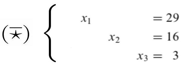
Par le théorème, \((\star)(\bar{\star})\) ont le même ensemble de solution. On voit que la solution de \((\bar{\star})\) est le triplet \((29 ; 16 ; 3) \Longrightarrow\) c’est l’uniaue solution de \((\star)\).
\(\textbf{Exemple 3.2}\) Soit le système
$$
(\star)\left\{\begin{array}{c}
x_{1}+x_{2}-2 x_{3}=1 \\
-2 x_{1}+x_{2}+x_{3}=4
\end{array}\right.
$$
\(L_{2} \longleftarrow L_{2}+2 L_{1}\)
$$
\left\{\begin{array}{c}
x_{1}+x_{2}-2 x_{3}=1 \\
3 x_{2}-3 x_{3}=6
\end{array}\right.
$$
\(L_{2} \longleftarrow \frac{1}{3} L_{2}\)
$$
(\bar{\star})\left\{\begin{array}{c}
x_{1}+x_{2}-2 x_{3}=1 \\
x_{2}-x_{3}=2
\end{array}\right.
$$
\(\textbf{Remarque : }\) On peut choisir \(x_{3}\), puis exprimer \(x_{2}\) et \(x_{1}\) uniquement en fonction de \(x_{3}\).
Fixons \(x_{3}\). Alors, de \(L_{2}\) on obtient:
$$
x_{2}=2+x_{3}
$$
On remplace dans \(L_{1}\) :
$$
\begin{aligned}
x_{1} & =1+2 x_{3}-x_{2} \\
& =1+2 x_{3}-\left(2+x_{3}\right) \\
& =-1+x_{3}
\end{aligned}
$$
Donc l’ensemble des solutions de \((\star)\) peut être décrit de la manière suivante :
C’est l’ensemble des triplets \(\left(x_{1}, x_{2}, x_{3}\right)\), où
-
\(x_{3}\) est libre (on peut le choisir),
une fois choisi \(x_{3}\), prendre
$$
\begin{aligned}
& x_{2}=2+x_{3} \\
& x_{1}=-1+x_{3}
\end{aligned}
$$
\(\longrightarrow\left\{\left(x_{1}, x_{2}, x_{3}\right) \mid x_{3} \in \mathbb{R}\right.\) libre, et \(\left.x_{2}=2+x_{3}, x_{1}=-1+x_{3}\right\}\)
$$
x_{3} \longleftrightarrow t
$$
\(\longrightarrow\{(-1+t, 2+t, t) \mid t \in \mathbb{R}\) libre \(\}\)
Notation Matricielle des systèmes linéaires
Toutes les opérations se font sur les coefficients \(\longrightarrow\) pour gagner du temps, on évite de toujours récrire ” \(x_{1}, x_{2}, \ldots, x_{n}\) ” en introduisant deux matrices associées à un système:
On peut présenter un système linéaire par une matrice appelée matrice associée du système où les coefficients de chaque inconnue ont été alignés verticalement dans une colonne de la matrice.
$$
\left\{\begin{array}{c}
a_{1,1} x_{1}+a_{1,2} x_{2}+\cdots+a_{1, n} x_{n}=b_{1} \\
a_{2,1} x_{1}+a_{2,2} x_{2}+\cdots+a_{2, n} x_{n}=b_{2} \\
\vdots \\
\vdots \\
a_{m, 1} x_{1}+a_{m, 2} x_{2}+\cdots+a_{m, n} x_{n}=b_{m}
\end{array} \Longrightarrow\left[\begin{array}{ccccc}
a_{11} & a_{12} & a_{13} & \ldots & a_{1 n} \\
a_{21} & a_{22} & a_{23} & \ldots & a_{2 n} \\
a_{31} & a_{32} & a_{33} & \cdots & a_{3 n} \\
\vdots & \vdots & \vdots & \ddots & \vdots \\
a_{m 1} & a_{m 2} & a_{m 3} & \ldots & a_{m n}
\end{array}\right]\right.
$$
a matrice augmentée ( ou complète) d’un système
La matrice augmentée ( ou complète) d’un système s’obtient en adjoignant à la matrice associée du système la colonne contenant les constantes des seconds membres de chaque équation.
$$
\left(\begin{array}{ccccc|c}
a_{11} & a_{12} & a_{13} & \ldots & a_{1 n} & b_{1} \\
a_{21} & a_{22} & a_{23} & \ldots & a_{2 n} & b_{2} \\
a_{31} & a_{32} & a_{33} & \ldots & a_{3 n} & b_{3} \\
\vdots & \vdots & \vdots & \ddots & \vdots & \vdots \\
a_{m 1} & a_{m 2} & a_{m 3} & \ldots & a_{m n} & b_{m}
\end{array}\right)
$$
Le coefficient principal d’une ligne
Dans une matrice \(m \times n\) le coefficients principal d’une ligne (non-nulle) est le premier coefficient \(a_{i j}\) non-nul rencontré en partant depuis la gauche.
Une matrice est échelonnée si
\(\triangleright\) Une matrice est échelonnée, si :
-
Tout les ligne entièrement nulles sont tout en bas.
Dans chaque ligne non-nulle, le coefficient principal est strictement à droite du coefficient principal de la ligne du dessus.
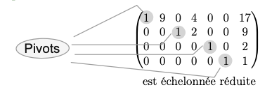
\(\triangleright\) On dit qu’une matrice est échelonnée réduite si elle est échelonnée et si de plus :
-
Tous les coefficients principaux valent 1 ( sont appelés pivots)
Chaque pivot est le seul coefficient non nul de sa colonne (colonne pivot).
\(\textbf{Exemple 4.1}\)
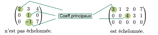
\(\textbf{Exemple 4.2}\)
\(\textbf{Théorème 4.1}\)
\(\triangleright\) Tout matrice \(A \in M_{m, n}(\mathbb{R})\) peut transformer en une matrice échelonnée, à l’aide d’une suite finie d’opérations élémentaires.
(Le résultat peut dépendre du choix des opérations.)
\(\triangleright\) Tout matrice \(A \in M_{m, n}(\mathbb{R})\) peut transformer en une matrice échelonnée réduite, à l’aide d’une suite finie d’opérations élémentaires.
(Le résultat ne dépend pas du choix des opérations.)
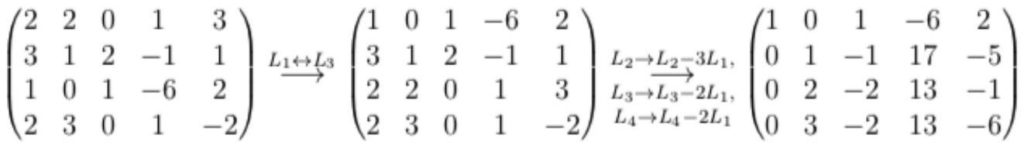
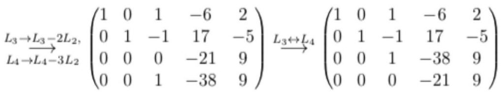
\(\textbf{Exemple 4.3}\) Échelonner et réduire la matrices suivante
$$
B=\left(\begin{array}{ccccc}
2 & 2 & 0 & 1 & 3 \\
3 & 1 & 2 & -1 & 1 \\
1 & 0 & 1 & -6 & 2 \\
2 & 3 & 0 & 1 & -2
\end{array}\right) \in M_{4 \times 5}(\mathbb{R})
$$
Solution :
$$
\begin{aligned}
& \stackrel{L_{4} \rightarrow-\frac{1}{21} L_{4}}{\longrightarrow}\left(\begin{array}{ccccc}
1 & 0 & 1 & -6 & 2 \\
0 & 1 & -1 & 17 & -5 \\
0 & 0 & 1 & -38 & 9 \\
0 & 0 & 0 & 1 & -\frac{3}{7}
\end{array}\right) \stackrel{L_{3} \rightarrow L_{3}+38 L_{4}}{\longrightarrow}\left(\begin{array}{ccccc}
1 & 0 & 1 & -6 & 2 \\
0 & 1 & -1 & 17 & -5 \\
0 & 0 & 1 & 0 & -\frac{51}{7} \\
0 & 0 & 0 & 1 & -\frac{3}{7}
\end{array}\right) \\
& \stackrel{L_{2} \rightarrow L_{2}+L_{3}}{\longrightarrow}\left(\begin{array}{ccccc}
1 & 0 & 1 & -6 & 2 \\
0 & 1 & 0 & 17 & -\frac{86}{7} \\
0 & 0 & 1 & 0 & -\frac{51}{7} \\
0 & 0 & 0 & 1 & -\frac{3}{7}
\end{array}\right) \stackrel{L_{2} \rightarrow L_{2}-17 L_{4}}{\longrightarrow}\left(\begin{array}{ccccc}
1 & 0 & 1 & -6 & 2 \\
0 & 1 & 0 & 0 & -5 \\
0 & 0 & 1 & 0 & -\frac{51}{7} \\
0 & 0 & 0 & 1 & -\frac{3}{7}
\end{array}\right) \\
& \stackrel{L_{1} \rightarrow L_{1}-L_{3}}{\longrightarrow}\left(\begin{array}{ccccc}
1 & 0 & 0 & -6 & \frac{65}{7} \\
0 & 1 & 0 & 0 & -5 \\
0 & 0 & 1 & 0 & -\frac{51}{7} \\
0 & 0 & 0 & 1 & -\frac{3}{7}
\end{array}\right) \stackrel{L_{1} \rightarrow L_{1}+6 L_{4}}{\longrightarrow}\left(\begin{array}{ccccc}
1 & 0 & 0 & 0 & \frac{47}{7} \\
0 & 1 & 0 & 0 & -5 \\
0 & 0 & 1 & 0 & -\frac{51}{7} \\
0 & 0 & 0 & 1 & -\frac{3}{7}
\end{array}\right) .
\end{aligned}
$$
\(\textbf{Exemple 4.4}\)
\((\star)\left\{\begin{array}{c}x_{1}+x_{2}=5 \\ 2 x_{1}+2 x_{2}=11\end{array} \longrightarrow\left(\begin{array}{cc|c}1 & 1 & 5 \\ 2 & 2 & 11\end{array}\right) \longrightarrow\left(\begin{array}{ll|l}1 & 1 & 5 \\ 0 & 0 & 1\end{array}\right) \longrightarrow(\bar{\star})\left\{\begin{array}{c}x_{1}+x_{2}=5 \\ 0=1\end{array}\right.\right.\).
Le système \((\bar{\star})\) n’ pas de solution \(\Longrightarrow(\star)\) n’en a pas non plus.
\(\textbf{Exemple 4.5}\)
$$
\left\{\begin{aligned}
3 x_{2}-6 x_{3}+6 x_{4}+4 x_{5} & =-5 \\
3 x_{1}-7 x_{2}+8 x_{3}-5 x_{4}+8 x_{5} & =9 \\
3 x_{1}-9 x_{2}+12 x_{3}-9 x_{4}+6 x_{5} & =15
\end{aligned}\right.
$$
La matrice augmentée du système est :
$$
\begin{aligned}
& \left(\begin{array}{ccccc|c}
0 & 3 & -6 & 6 & 4 & -5 \\
3 & -7 & 8 & -5 & 8 & 9 \\
3 & -9 & 12 & -9 & 6 & 15
\end{array}\right) \longrightarrow\left(\begin{array}{ccccc|c}
1 & 0 & -2 & 3 & 0 & -24 \\
0 & 1 & -2 & 2 & 0 & -7 \\
0 & 0 & 0 & 0 & 1 & 4
\end{array}\right)
\end{aligned}
$$
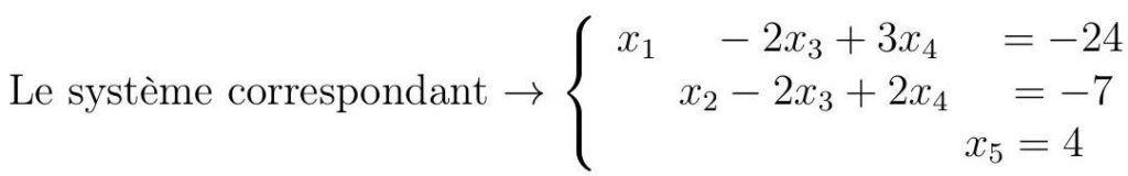
\(x_{3}\) et \(x_{4}\) sont libres. Les autres sont liées à \(x_{3}\),
$$
\begin{aligned}
& x_{1}=-24+2 x_{3}-3 x_{4} \\
& x_{2}=-7+2 x_{3}-2 x_{4} \\
& x_{5}=4
\end{aligned}
$$
Matrices Échelonnées (Réduites)
Vous pouvez saisir des équations mathématiques via LaTeX comme ceci : \[ Votre équation \].
Par exemple : \[E=mc^2\] donnera : \[E=mc^2\]
Pour en savoir plus sur LaTeX, consultez ce tutoriel. (Anglais)
Laisser un commentaire
Vous devez vous connecter pour publier un commentaire.
Vous pouvez saisir des équations mathématiques via LaTeX comme ceci : \[ Votre équation \]. Par exemple :
\[E=mc^2\]donnera : \[E=mc^2\]Pour en savoir plus sur LaTeX, consultez ce tutoriel. (Anglais)